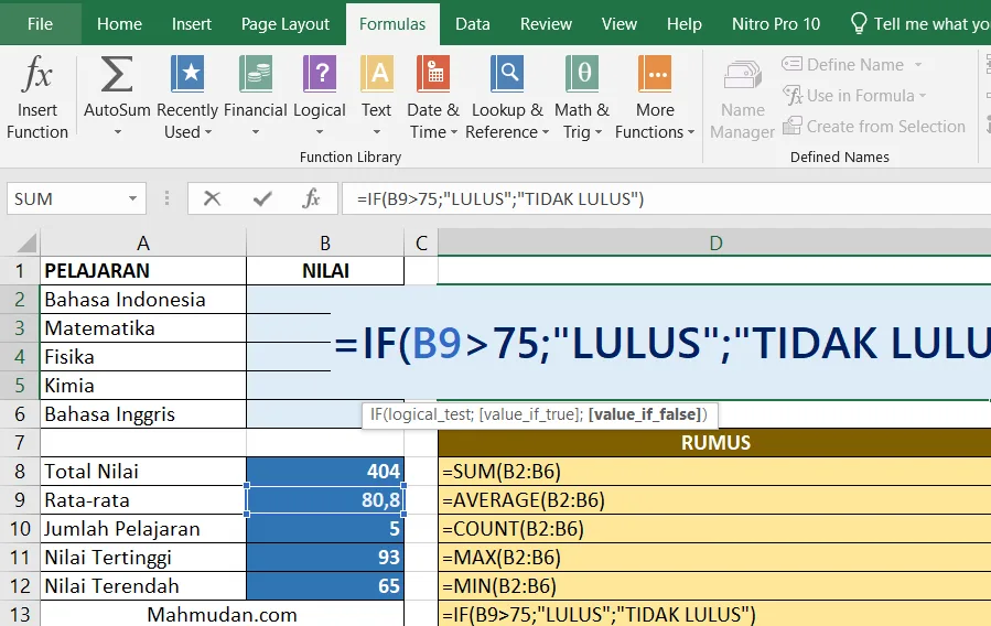
41 Important Excel Formula Functions in Work

By mastering 41 this important Excel formula function, You will experience increased effectiveness and accuracy of results. Proper use of Excel formula functions can avoid errors and thus increase productivity in your work.

The work results obtained will not be optimal when working with Excel don't use formulas. Excel's formula function provides great benefits in calculating, analyze, and present data efficiently. By using the formula, You can do math calculations, statistics, logic, and much more easily and accurately.

You can create formulas and use Excel's built-in functions to perform calculations and solve problems. The following are important Excel formula functions in work and examples of their use.

List of contents

Excel Formula Functions by Category

Every formula written in Excel must begin with an equal sign (” = “).

Mathematics

SUM Adds a range of numbers. Example: =SUM(A1:A5)
MAX Returns the highest value in a number range. Example: =MAX(A1:A5)
MIN Returns the lowest value in a number range. Example: =MIN(A1:A5)
ROUND Rounds a number to a specified number of digits. Example: =ROUND(A1;2)
ROUNDUP Rounds a number up to a specified number of digits Example: =ROUNDUP(A1;2)
ROUNDDOWN Rounds a number down to a specified number of digits. Example: =ROUNDDOWN(A1;2)
RAND Returns an intermediate random number 0 and 1. Example: =RAND()
SUMIF Sums cells in a range that meet certain criteria. Example: =SUMIF(A1:A5;”>10″)
SUMIFS Sums cells in a range that meet certain criteria. Example: =SUMIFS(A1:A5,”>10″,B1:B5,”<20″)

Statistics

AVERAGE Calculates the average of a range of numbers. Example: =AVERAGE(A1:A5)
COUNT Counts the number of cells in a range that contain numbers. Example: =COUNT(A1:A5)
COUNTIF Counts the number of cells in a range that meet certain criteria. Example: =COUNTIF(A1:A5;”>10″)
AVERAGEIF Calculates the average of cells in a range that meet certain criteria. Example: =AVERAGEIF(A1:A5;”>10″)
COUNTIFS Counts the number of cells in a range that meet some specified criteria. Example: =COUNTIFS(A1:A5;”>10″,B1:B5;”<20″)
RANK Returns the rank of a number in a number range; Example: =RANK(A1;A2:A5)
AVERAGEIFS Calculates the average of cells in a range that meet some specified criteria. Example: =AVERAGEIFS(A1:A5,”>10″,B1:B5;”<20″)

Logical

IF Returns one value if a condition is true and another value if it is false. Example: =IF(A1>10;”Yes”;”No”)
AND Returns TRUE if all arguments are true. Example: =AND(A1>10;BI<20)
OR Returns TRUE if any argument is true. Example: = OR(A1>10;BI<20)
NOT Returns the inverse of a logical value. Example: =NOT(A1>10)
IFERROR Returns a value if the formula evaluates to error: if not, returns the formula result; Example: =IFERROR(A1/B1;”Error”)

Date And Time

TODAY Returns the current date. Example: =TODAY()
NOW Returns the current date and time. Example: =NOW()
DATE Returns the date serial number . Example: =DATE(2022;4;6)
TIME Returns the time serial number. Example: =TIME(12;30;0)

Search and Reference

VLOOKUP Looks up a value in a table and returns the corresponding value in the same row Example: =VLOOKUP(A1;A2:B5;2;FALSE)
SEARCH Looks up a value in a table and returns the corresponding value in the same column Example: =LOOKUP(A1;A2:B5;2;FALSE)
INDEX Returns a value or reference to a value from within a table or range Example: =INDEX(A1:B5;3;2)
MATCH Searches for a value in a range and returns the position of the value in that range Example: =MATCH(A1;A2:A5;0)
CHOOSE Selects a value from a list of values based on a specified position Example: =CHOOSE(2;”Monday”;”Tuesday”;”Wednesday”)

Text

CONCAT Combines two or more text strings into one string. Example: =CONCATENATE(“Hello”;””;”World”)
LEFT Returns the specified number of characters from the left of the text string. Example: =LEFT(A1;5)
RIGHT Returns the specified number of characters from the right of the text string. Example: =RIGHT(A1;5)
MID Returns the specified number of characters from the middle of the Example text string: =MID(A1;3;5)
LEN Returns the length of a text string. Example: =LEN(A1)
SUBSTITUTE Replaces text in a text string with new text. Example: =SUBSTITUTE(A1;”old”;”new”)
TRIM Removes leading and trailing spaces from a text string. Example: =TRIM(A1)
PROPER Capitalize the first letter of each word in the text string. Example: =PROPER(A1)
LOWER Converts all letters in text to lowercase. Example: =LOWER(A1)
UPPER Converts all letters in text to uppercase. Example: =UPPER(A1)
TEXT Converts a value to text in a specific format. Example: =TEXT(A1;”0;00″)

Combining Excel Formula Functions

On Microsoft Excel, You can create formulas using a combination of several functions with basic mathematical operations such as summation, subtraction and multiplication. Example:

Addition and Subtraction Formulas:

=SUM(A1:A5)-(B1+C3+D6)

Formula for Calculating Age:

=CONCATENATE(DATEDIF(A1;NOW();”Y”);” Year “;DATEDIF(A1;NOW();”YM”);” Month “;DATEDIF(A1;NOW();”MD”);” Day”)

That's it 41 important and useful Excel formula functions that can be shared with you.

Hope it is useful.